Optimal-Portfolio-Allocation

🚀 Multi-Criteria Portfolio Optimizer: Monte Carlo Allocation Engine

This project provides a robust Python solution for determining optimal portfolio allocations based on a set of user-defined stock tickers and historical data. Utilizing the Monte Carlo Simulation technique, this tool identifies portfolios that excel across several key risk-adjusted metrics, moving beyond just the traditional Sharpe Ratio to offer a more nuanced view of capital efficiency and risk management.

⚙️ Core Technical Architecture and Methodology

The system is built around the financial engineering principle of the Efficient Frontier, computationally searching the space of all possible weight combinations to find the highest return for a given level of risk (volatility).

1. Data Ingestion and Financial Preprocessing

The application leverages the yfinance library for seamless acquisition of historical stock price data.

Data Source: Fetches adjusted closing prices for the specified list of TICKERS.
Transformation: Calculates daily percentage returns (data.pct_change()).
Annualization: Establishes the annualization factor (default: 252 trading days) to calculate the Annualized Mean Returns Vector and the Annualized Covariance Matrix ($\Sigma$). This matrix is critical as it captures the interplay (correlation/co-variance) between the assets, forming the backbone of portfolio volatility calculation: $\sigma_p = \sqrt{\mathbf{w}^T \mathbf{\Sigma} \mathbf{w}}$.

2. Monte Carlo Simulation

The core optimizer runs a high-volume Monte Carlo Simulation (default: 50,000 iterations). In each run, a set of random weights ($\mathbf{w}$) is generated and normalized ($\sum w_i = 1$). For every simulated portfolio, five key metrics are computed:

Annualized Return ($\mu_p$)
Annualized Volatility ($\sigma_p$)
Sharpe Ratio
Sortino Ratio
Calmar Ratio

3. Advanced Risk-Adjusted Metrics

This optimizer provides enhanced insights by calculating metrics that specifically target downside or drawdown risk, offering a superior measure of portfolio quality compared to metrics relying solely on total volatility ($\sigma_p$):

Metric	Calculation Focus	Technical Implementation
Sharpe Ratio	Return per unit of Total Volatility.	$(\mu_p - R_f) / \sigma_p$
Sortino Ratio	Return per unit of Downside Deviation.	$(\mu_p - R_f) / \text{Downside Deviation}$
Calmar Ratio	Return relative to the Maximum Drawdown.	$\mu_p / \text{Max Drawdown}$

The implementation of Max Drawdown involves calculating the cumulative returns and tracking the difference between the running peak and the trough that follows. Downside Deviation is calculated as the volatility of only the returns that fall below a Minimum Acceptable Return (MAR).

✨ Identifying the Optimal Portfolios

The simulation results are collated into a pandas.DataFrame, enabling efficient identification of four critical benchmark portfolios:

Max Sharpe Ratio Portfolio: The ideal point on the classic Efficient Frontier.
Min Volatility Portfolio: The Global Minimum Variance Portfolio (GMVP), which carries the lowest possible risk for the selected assets.
Max Sortino Ratio Portfolio: The most effective portfolio in mitigating downside risk.
Max Calmar Ratio Portfolio: The most effective portfolio for capital preservation against significant historical losses.

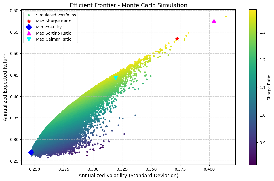
🖼️ Visualization: The Efficient Frontier

The results are beautifully visualized using matplotlib. The plot maps the entire simulated universe in the Return vs. Volatility space. Portfolios are color-coded by their Sharpe Ratio for instant insight into efficiency, and the four optimal portfolios are highlighted with distinct markers to pinpoint the best allocations according to each specific risk metric.

🛠️ Getting Started

Prerequisites

pip install yfinance pandas numpy matplotlib

Configurations

TICKERS = ['META', 'MSFT', 'NVDA', 'AAPL', 'AMZN', 'GOOG']
RISK_FREE_RATE = 0.02 # Annual risk-free rate (e.g., 2%)
NUM_PORTFOLIOS = 50000

Results

The compositions:

--- Portfolio Optimization Results (50000 Simulations) ---
Tickers: META, MSFT, NVDA, AAPL, AMZN, GOOG
Risk-Free Rate: 2.00%

--- Portfolio with MAXIMUM SHARPE RATIO ---
Annual Return:        53.43%
Annual Volatility:    37.22%
Sharpe Ratio:         1.3818
Sortino Ratio:        1.3912
Calmar Ratio:         0.9654

Allocation Weights:
  GOOG : 62.60%
  MSFT : 16.49%
  META : 8.55%
  NVDA : 6.24%
  AMZN : 6.02%
  AAPL : 0.10%

--- Portfolio with MINIMUM VOLATILITY ---
Annual Return:        26.96%
Annual Volatility:    24.69%
Sharpe Ratio:         1.0108
Sortino Ratio:        0.9785
Calmar Ratio:         0.7279

Allocation Weights:
  NVDA : 31.11%
  META : 29.35%
  AMZN : 27.73%
  MSFT : 10.77%
  AAPL : 0.62%
  GOOG : 0.42%

--- Portfolio with MAXIMUM SORTINO RATIO ---
Annual Return:        57.60%
Annual Volatility:    40.40%
Sharpe Ratio:         1.3763
Sortino Ratio:        1.4095
Calmar Ratio:         0.9757

Allocation Weights:
  GOOG : 73.81%
  AMZN : 8.52%
  MSFT : 8.11%
  NVDA : 6.57%
  META : 2.92%
  AAPL : 0.07%

--- Portfolio with MAXIMUM CALMAR RATIO ---
Annual Return:        44.29%
Annual Volatility:    31.96%
Sharpe Ratio:         1.3232
Sortino Ratio:        1.3104
Calmar Ratio:         1.0056

Allocation Weights:
  META : 49.95%
  GOOG : 41.53%
  NVDA : 4.10%
  MSFT : 2.49%
  AMZN : 1.46%
  AAPL : 0.48%

The Efficient Frontier Plot:

Back to Index