Quantitative-Fund-Portfolio-Performance-Simulation-and-Analysis

📈 Quantitative Portfolio Performance Simulation and Analysis

This repository hosts a robust Python simulation designed to quantitatively backtest the performance of a custom-defined stock portfolio against a major market index over a specified historical period.

The portfolio’s asset allocation—defined by the stock tickers and their corresponding weights—is sourced directly from a data-driven Optimal Portfolio Allocation model developed in a prior project: handiko/Optimal-Portfolio-Allocation.

This project focuses on the technical execution of the simulation, robust data reconciliation, and the computation of key, annualized performance metrics, providing a comprehensive quantitative comparison.

🛠️ Technical Overview and Methodology

1. Data Acquisition and Preprocessing

The simulation leverages the yfinance library for fetching historical market data, specifically adjusted daily closing prices.

Data Source: Adjusted daily closing prices are downloaded for the specified portfolio constituents (e.g., META, MSFT, NVDA, etc.) and the chosen Comparison Index (e.g., NQ=F).
Time Horizon: The simulation is configured for a lump-sum investment over a customizable lookback period (default is 10 years ending on a specified END_DATE).
Data Alignment: A critical step is the reconciliation and alignment of the daily returns. Daily returns for all individual stocks and the comparison index are calculated, and then both series are intersected (common_index) to ensure they cover the exact same set of trading days. This guarantees a fair, like-for-like performance comparison.

2. Portfolio and Index Return Calculation

Portfolio Returns:

The simulation assumes a buy-and-hold strategy based on the initial allocation (no rebalancing). The daily portfolio return ($\text{Return}_p$) is calculated as a weighted sum of the individual stock daily returns ($\text{Return}_i$):

\[\text{Return}_p = \sum_{i=1}^{N} (w_i \times \text{Return}_i)\]

Where $w_i$ is the fixed capital weight of stock $i$.

Balance Growth Calculation:

The portfolio balance growth reflects how an INITIAL_CAPITAL (e.g., $10,000) would have grown over the period:

Individual Stock Growth: The cumulative return ($C_i$) for each stock is computed from its daily returns.
Portfolio Balance: The total value is the sum of the initial capital allocated to each stock multiplied by its cumulative return: $\text{Balance}_p = \sum_{i=1}^{N} (w_i \times \text{Initial Capital} \times C_i)$
Index Balance: The comparison index’s cumulative growth is scaled by the INITIAL_CAPITAL to match the portfolio’s starting value for the visual comparison.

3. Quantitative Performance Metrics (Annualized)

Metric	Description	Formula Highlights
Sharpe Ratio	Risk-adjusted return for unit of total volatility.	$\frac{\text{Mean}(\text{Excess Returns})}{\text{StdDev}(\text{Excess Returns})} \times \sqrt{252}$
Sortino Ratio	Risk-adjusted return focusing only on downside volatility (returns below $\text{Daily RFR}$).	$\frac{\text{Mean}(\text{Returns}) - \text{Daily RFR}}{\text{StdDev}(\text{Downside Returns})} \times \sqrt{252}$
Calmar Ratio	Measures return (Compound Annual Growth Rate, CAGR) relative to Maximum Drawdown (MDD).	$\frac{\text{CAGR}}{	\text{Max Drawdown}	}$
Max Drawdown (MDD)	The largest peak-to-trough decline over the entire period.	$\min\left(\frac{\text{Cumulative Wealth}}{\text{Peak Cumulative Wealth}}\right) - 1$

🚀 Getting Started

To run this backtesting simulation, you will need to install the core dependencies:

pip install yfinance pandas numpy matplotlib tabulate

Results

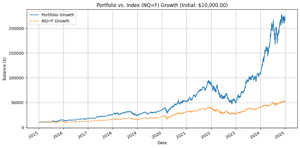
Portfolio performance against the Nasdaq Index (NQ=F)

======================================================================
Simulation Period: 2015-01-06 to 2024-12-31
Initial Investment: $10,000.00
======================================================================
| Metric        | Portfolio   | NQ=F       |
|:--------------|:------------|:-----------|
| Final Balance | $214,683.16 | $51,700.87 |
| Total Return  | 2046.83%    | 417.01%    |
| Sharpe Ratio  | 0.9722      | 0.7663     |
| Sortino Ratio | 1.3027      | 0.9774     |
| Calmar Ratio  | 0.5859      | 0.5031     |

Portfolio performance chart:

Back to Index