Machine Learning Stock Backtesting Framework
Can a machine learning model beat buy-and-hold on Indonesian stocks?
This project builds, tests, and rigorously evaluates a trading strategy powered by XGBoost — one of the most battle-tested ML algorithms in quantitative finance.
What Is This Project?
Imagine you could teach a computer to study 15 years of stock price history — every wiggle, every trend, every indicator traders use — and learn when a stock is most likely to rise in the next few days. That’s exactly what this framework does.
It trains an XGBoost machine learning model on historical stock data, then simulates trading based on that model’s signals, and finally presents a full performance dashboard so you can judge for yourself: is this strategy worth anything in the real world?
The framework is built with a trader’s mindset: it accounts for realistic trade execution, transaction costs, and — critically — makes sure the model never “cheats” by peeking at future data during training.
Goals
| Goal | How It’s Addressed |
|---|---|
| Predict short-term price direction | XGBoost classifier on 80+ technical features |
| Avoid overfitting (the #1 failure of ML in trading) | Walk-forward retraining + purged cross-validation + feature selection |
| Simulate real-world trading | Execution at next day’s open price + transaction costs |
| Measure true out-of-sample performance | Strict train / validation / hold-out data splits |
| Understand why the model trades | Feature importance chart |
How It Works — Step by Step
1. Data Download
Stock price data (OHLCV: Open, High, Low, Close, Volume) is downloaded automatically via yfinance for any ticker — Indonesian stocks (.JK), US stocks, or any market supported by Yahoo Finance. The default lookback is 15 years.
2. Feature Engineering (~80 Technical Indicators)
Raw prices are transformed into features that describe the current market state. These are the same signals technical traders use, but fed to a machine instead of human eyes:
- Trend features — price relative to SMA(5/10/20/50/100/200), EMA crossovers, MACD, ADX
- Momentum features — rate of change (ROC), past returns (1d to 63d), RSI (7/14/21)
- Volatility features — rolling standard deviation, ATR (Average True Range), Bollinger Band width
- Volume features — OBV (On-Balance Volume), MFI (Money Flow Index), volume ratio vs. moving average
- Statistical features — rolling skewness, kurtosis, 52-week high/low deviation
- Calendar features — day of week, month (captures seasonality)
All features are normalized relative to price (e.g., (Close - SMA) / SMA) so they stay comparable across different stocks and time periods.
3. Labeling
The model learns to predict: “Will this stock rise by at least X% over the next N days?”
- Buy-Only mode: Label =
1(buy signal) if the stock gains >label_pct% inforward_daystrading days, else0(stay flat). - Buy-Sell mode: Adds a
-1label (sell/short signal) for stocks expected to drop.
The default is 3-day horizon with a 1% threshold — asking the model to predict meaningful near-term moves.
4. Data Splitting (The Most Critical Step)
The dataset is split chronologically — never randomly — into three non-overlapping periods:
|──────────── In-Sample (60%) ────────────|── Validation (20%) ──|── Hold-Out (20%) ──|
         Model is trained here              Hyperparameter tuning    True test of reality
- In-Sample: Where the model learns patterns.
- Validation: Used to stop training early (prevent overfitting) and tune thresholds.
- Hold-Out: The model has never seen this data. Performance here is the only honest measure.
Why this matters: Most “backtests” you see online are overfit — the model was implicitly tuned on the test data. This framework enforces a strict wall between learning and evaluation.
5. Model Training
XGBoost (eXtreme Gradient Boosting) is an ensemble of decision trees that learns from its own mistakes iteratively. It’s the algorithm behind many winning solutions in quantitative trading competitions.
Key anti-overfitting measures baked in:
| Parameter | Setting | Effect |
|---|---|---|
max_depth = 3 |
Shallow trees | Can’t memorize noise |
learning_rate = 0.02 |
Small steps | Generalizes better |
colsample_bytree = 0.5 |
Use 50% of features per tree | Forces diversity |
min_child_weight = 8 |
Need 8+ samples per leaf | Avoids spurious splits |
reg_alpha/lambda |
L1 + L2 regularization | Penalizes complexity |
early_stopping_rounds = 40 |
Stop if val loss doesn’t improve | Prevents overtraining |
scale_pos_weight |
Auto class balancing | Handles rare buy signals |
6. Purged Walk-Forward Cross-Validation
Standard k-fold cross-validation is broken for time series — it lets the model train on data after the test period, leaking future information.
This framework uses Purged + Embargoed Walk-Forward CV:
- Folds are strictly ordered in time (no shuffling).
- A 5-row embargo gap is added between training and validation folds.
This gap removes rows that might share information with the test period (since a 3-day forward label computed on day T overlaps with prices on days T+1 through T+3).
The output is a CV AUC score — a leakage-free estimate of how well the model distinguishes buy opportunities from non-opportunities.
7. Feature Selection
Training on all 80+ features often hurts performance — noise overwhelms signal. After initial training, the framework ranks features by XGBoost importance and keeps only the top-K (default: 15). The model is then retrained on this curated feature set.
In the example dashboard (BBCA.JK), the top features were SMA deviations, EMA distances, rate-of-change, MACD, and Bollinger Band position — classic trend-following and mean-reversion signals.
8. Walk-Forward Retraining (Expanding Window)
Markets change. A model trained in 2015 may be completely wrong in 2023. To handle this:
- The model starts with knowledge up to the end of the in-sample period.
- Every N months (default: 6), the model retrains from scratch on all data seen so far.
- It then predicts only the next chunk of data — never the future.
This is how professional quant funds operate. It’s the difference between a static snapshot and a living, adapting system.
|─ IS train ─|── retrain ──|── retrain ──|── retrain ──|
              ↓              ↓              ↓
           predict →      predict →      predict →
9. Signal Generation
Raw probability outputs from the model are converted to trading signals using a dual filter:
- Percentile rank filter: Only fire a BUY when the model’s confidence is in the top 25% of all signals (so it only acts on its strongest convictions).
- Minimum probability floor: The raw buy probability must also exceed 0.40 (avoids acting on marginal signals near the 50/50 boundary).
An optional SMA regime filter (e.g., SMA-200) can restrict longs to bull markets only, significantly reducing drawdown.
10. Realistic Backtest Engine
The backtest is designed to be as close to real trading as possible:
- Signal at Close[T] → Execute at Open[T+1]: You see the signal after market close, then execute at the following morning’s open. No cheating with same-bar fills.
- Transaction costs: Default 5 basis points (0.05%) per trade, applied on position changes.
- Position tracking: Cumulative equity curve, drawdown, and per-trade statistics are all computed.
How to Read the Dashboard
The dashboard produced by the script has 6 panels:
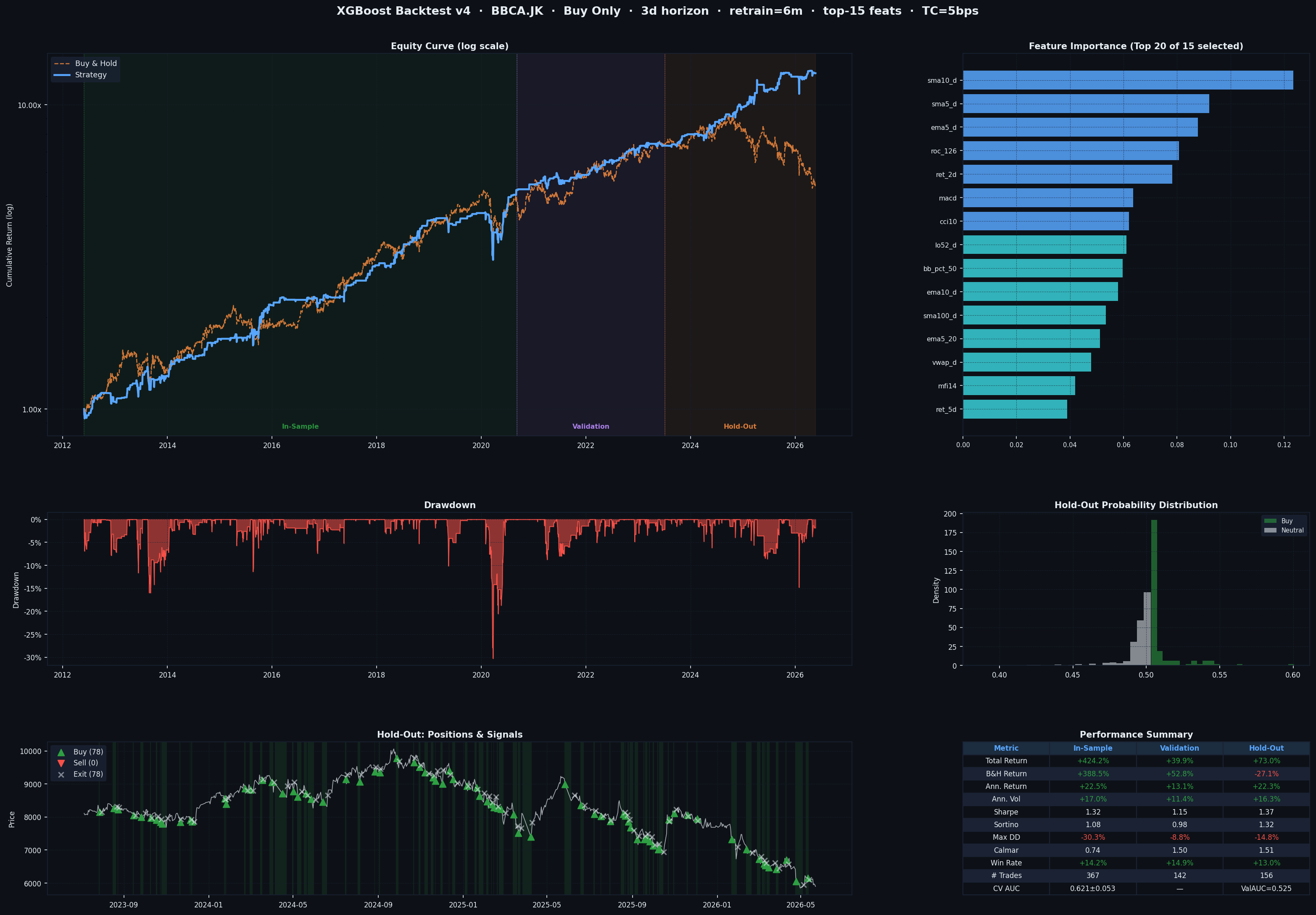
Top-Left: Equity Curve (Log Scale)
- Blue line = Strategy performance
- Orange dashed line = Buy & Hold benchmark
- Three shaded regions mark In-Sample, Validation, and Hold-Out periods
- Log scale lets you compare percentage gains fairly across time
You want the blue line to stay above orange, especially in the Hold-Out region — that’s the only part that counts.
Top-Right: Feature Importance
- Shows which of the top-15 selected features drive the model’s decisions
- Brighter blue = above-median importance
- In the BBCA example:
sma10_d(deviation from 10-day SMA) dominated — the model learned to buy pullbacks from trend.
Middle-Left: Drawdown
- Shows how far the strategy fell from its peak at any point in time
- Shallower and shorter drawdowns = better risk management
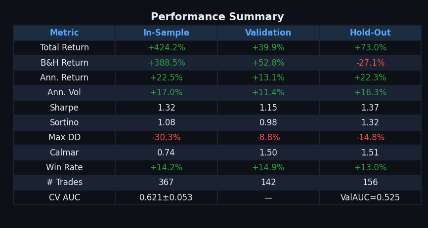
- A max drawdown of -14.8% on BBCA hold-out means the worst losing streak cut equity by ~15%
Middle-Right: Hold-Out Probability Distribution
- Shows the distribution of buy probabilities during the hold-out period
- Green = days where a BUY signal was fired
- Gray = neutral days
- A clean separation between the two clusters means the model is decisive
Bottom-Left: Hold-Out Positions & Signals
- Price chart overlaid with trade markers
-
🔺 Green triangles = BUY entries 🔻 Red triangles = SELL entries ✕ = exits - Green shading = periods when the strategy holds a long position
Bottom-Right: Performance Summary Table
| Metric | What It Means | Good Value |
|---|---|---|
| Total Return | Cumulative gain over the period | Higher than B&H |
| B&H Return | What you’d earn just holding | The benchmark to beat |
| Ann. Return | Annualized compound return | > 15% is strong |
| Ann. Vol | Annualized daily volatility | Lower = smoother ride |
| Sharpe | Return per unit of risk | > 1.0 is good, > 1.5 is great |
| Sortino | Like Sharpe but only penalizes downside volatility | > 1.0 is solid |
| Max DD | Worst peak-to-trough drawdown | Closer to 0% is better |
| Calmar | Ann. Return / Max Drawdown | > 1.0 means returns justify the risk |
| Win Rate | % of trading days that were profitable | Often 50–60% is fine with good Sharpe |
| # Trades | Total position changes (entries + exits) | Lower = less friction |
| CV AUC | Cross-validation discrimination score | > 0.55 is meaningful signal |
Installation & Usage
Requirements
pip install yfinance xgboost scikit-learn pandas numpy matplotlib joblib python-dateutil
Run
python ML_Stock_Backtest.py
The output will be:
- A printed performance table in the terminal
- A saved dashboard PNG:
xgb_backtest_dashboard.png - A saved model bundle:
xgb_{TICKER}_{MODE}_{N}d.pkl(for live use)
Configuration
Edit the CONFIG dict at the top of the file:
CONFIG = dict(
    ticker          = "BBCA.JK",   # Any Yahoo Finance ticker
    years           = 15,           # Years of history to download
    mode            = "buy_only",   # "buy_only" or "buy_sell"
    forward_days    = 3,            # Prediction horizon (trading days)
    label_pct       = 1.0,          # % move threshold to label as "buy"
    retrain_months  = 6,            # Walk-forward retraining frequency
    top_k_features  = 15,           # Feature selection cutoff
    regime_sma      = None,         # e.g. 200 → only buy above SMA(200)
    buy_pct         = 25,           # Top N% confidence percentile for BUY
    min_prob_floor  = 0.40,         # Minimum raw probability to trade
    transaction_cost_bps = 5,       # Round-trip cost in basis points
)
Important Caveats
This is a research and educational framework, not a live trading system. Before drawing conclusions:
- Past performance does not guarantee future results. Even a genuine edge can disappear as markets adapt.
- Hold-Out performance is the only honest signal. In-sample and validation numbers are expected to look good.
- Transaction costs matter more at high frequency. More trades = more friction. The default 5bps is optimistic for some brokers.
- This framework does not account for liquidity, slippage, or market impact — all of which matter for real execution.
- Always paper-trade first before committing real capital to any strategy derived from this analysis.
Key Design Decisions
| Decision | Rationale |
|---|---|
| XGBoost over deep learning | More robust on tabular data with limited samples; interpretable |
| Expanding window (not rolling) | Maximizes training data; avoids discarding early regime information |
| Percentile-rank signals (not raw probs) | Self-adjusting threshold; robust to distribution shift |
| Open-price execution | Removes look-ahead bias; more realistic than close-to-close |
| RobustScaler | Less sensitive to extreme outliers than StandardScaler |
scale_pos_weight |
Handles class imbalance without undersampling |
Repository Structure
├── ML_Stock_Backtest.py              # Main framework
├── README.md                         # This file
├── BBCA_JK_xgb_backtest_dashboard.png  # Example dashboard output
└── xgb_BBCA.JK_buy_only_3d.pkl      # Saved model bundle (after running)
License
MIT — use freely, contribute back if you improve it.
Built with Python · XGBoost · scikit-learn · yfinance · matplotlib